
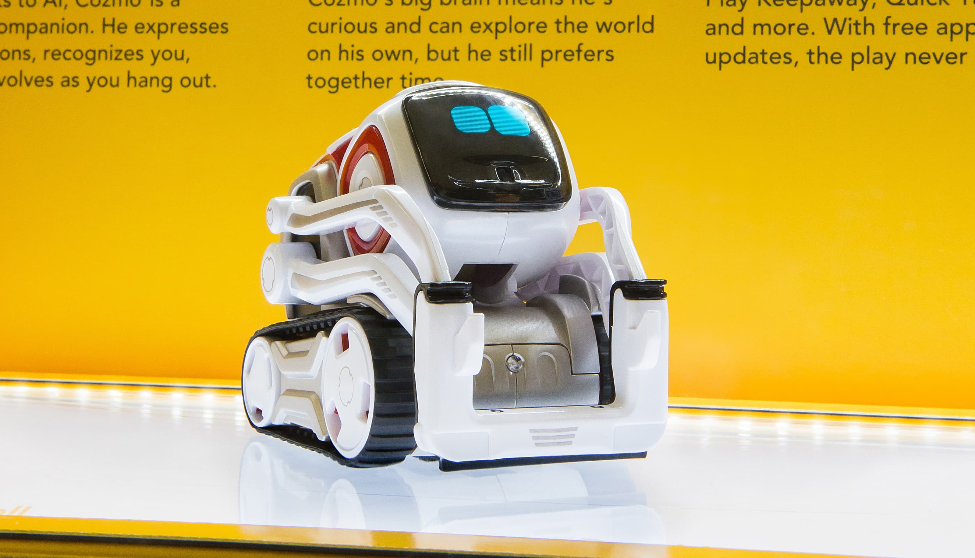
Anki Cozmo
Robotic Programming using Python and the Anki SDK
Using the Anki Cozmo, I carried out a number of projects each showcasing a different robotic programming technique.
Object Recognition
The first step in using the robot was to enable it to interpret it's visual percepts. This was done by configuring the embedded camera to constantly stream greyscale images and then extracting the features of the images to feed through a classifier. There were three classes in this case and the classification accuracy was boosted by predicting the class over a window of time. Rather than taking one picture, classifying it, and trusting this prediction, it is safer to do this over many images taken over a window of time. The ultimate prediction is then defined as the most commonly predicted class. Depending on what class the robot perceived, it would perform a task. These tasks included simple mechanisms like moving a cube from A to B, driving in a square, and driving in an S shape. Each task was performed by directly setting the speed and angle values for the robotic wheels. The code for forming the S shape is shown below.
						robot = sdk_conn.wait_for_robot()
						robot.drive_wheels(25, 75, duration = 5) # turn left
						robot.drive_wheels(75, 25, duration = 6) # turn right
Localization
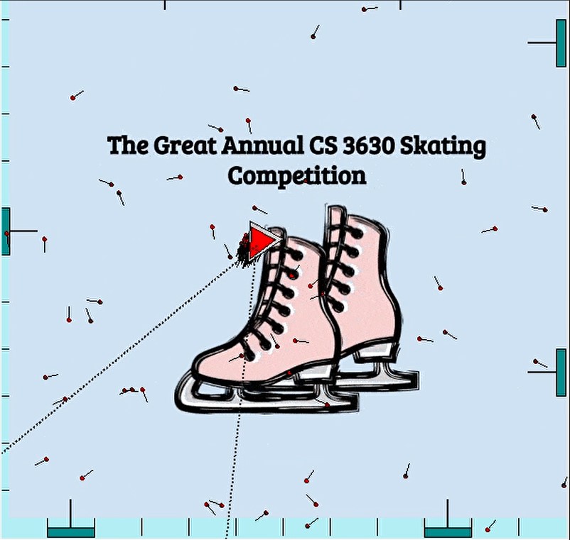
Next, the robot needed to be able to take in percepts and use them to localize itself in a 2D mapping. This was done using a particle filter to constantly update a probability distribution of where the robot is most likely located. We start with a few thousand particles, or prediction points, randomly distributed throughout the grid world with each particle object having an (x,y) position and a heading. As the algorithm performs motion and measurement updates, the particles start to clump together and place more confidence in a certain prediction. In the below picture, the red triangle is the true position while the grey triangle is the average positional guess of all the particles.

As the updates continue and the solution gets closer to convergence, the predicted location can be seen directly lining up with the ground truth location.
These updates were done by leveraging the robot's odometer readings. The motion update's purpose is to simulate movement of all the particles each time step. This is done by taking in a distance and direction to move, turning the particles to match the target heading, and moving the proper distance in that heading.
		# Motion Update
	            for i, _ in enumerate(motion_particles):
					prev_angle = motion_particles[i].h
					[xr , yr] = rotate_point(odom[0], odom[1], prev_angle)
					new_x  = motion_particles[i].x + xr
					new_y  = motion_particles[i].y + yr
					new_h  = motion_particles[i].h + odom[2]

					new_x, new_y, new_h = add_odometry_noise((new_x, new_y, new_h))

					motion_particles[i] = Particle(new_x,new_y,new_h)

				return motion_particles
For the measurement update, we can think of this as the particle population being refined. A gaussian probability density is calculated for each particle at this stage that is recorded amongst all particles, normalized, and then randomy sampled from to determine which particles should be kept around. The rest of the population is replaced with newly spawned, random particles. The PDF captures the differences between the robot's observed heading/position relative to a marker the robot camera sees and the relative heading/position expected by the robot with its current particle filter prediction. The simplified logit equation is seen below. If a particle is off screen after a motion update, it is immediately designated for replacement.

Path Planning
With the robot now armed with the ability to understand it's location in a grid world, the next challenge was to have the robot be able to plan a path to a goal point. The robot would know the world dimensions but would have to recognize any obstacles. This was done using RRTs, or Rapidly-exploring Random Trees, to first plan a path to the goal state assuming no obstacles are present and then sending the robot along that path. If the robot encountered an obstacle along the way through its camera, it woud stop and re-plan its path to the goal now taking the obstacle into consideration.
Under the hood, the RRT algorithm is somewhat simple. Each time step the robot randomly samples from all the locations in the grid world. Each current node in the tree has their euclidean distance to this random location calculated. The nearest node is then expanded towards the random node if no obstacles are preventing the link. We cap the maximum expansion distance here to reign in the expansion. As we progress through iterations, the tree eventually expands to the goal state and the tree can be backtraced to extract a path to the goal. This path is then smoothed by removing nodes where possible. For example, if nodes A and C can be connected by a straight line without hitting any obstacles, there is no need to keep node B around. A maximum link distance is still enforced to allow the robot to travel shorter, less error-prone distances at a time. Examples of my path planning algoritm with a known set of obstacles in the world can be seen below.
PID Control
For one last project, the robot was challenged with moving in a straight line as fast as it can to reach a designated 'parking' zone. The challenge here is that a block is placed just past the zone, requiring the robot to come to a precise stop despite coming in at a high speed. Furthermore, the robot needed to be robust to any disturbances it experienced along the way, adjusting its speed accordingly.

Using the robot's camera to record it's current position relative to the cube, the error between the robot's current position and the position marking the center of the parking zone was recorded. The time derivate as well as the sum of the errors over time were also tracked.
			while(not converged):

			    # Perceive Current Robot Position
				distance_away_x = cube_x - robot.pose.position.x

				# PID
				# Record time passed for time derivative
				time_passed = time.time() - prev_time
				prev_time = time.time() # Store for next calculations

				#Compute all error term values
				error = distance_away_x - 130 # 130 is the middle point of parking zone
				error_sum = error_sum + error
				error_deriv = (error - error_prev) / time_passed

				# Store current error for next calculations
				error_prev = error

				pid = (kp * error) + (kd * error_deriv) + (ki * error_sum)
				move(robot, pid, pid)
Looping until the robot reaches the goal state, this PID loop constantly adapts the robot speed to slow down steadily as it approaches the goal for a smooth parking job. The real challenge with this algorithm was the PID tuning of the proportional, derivative, and integral gains. I had started off with an eyeball approach, adjusting the gains as I saw issues manifest in the robot movement. For example, if the robot was getting to the goal too slowly I bumped up the proportional gain. If I saw oscillations around the parking space, I bumped up the derivative gain. This worked well, but was not perfect given the interactions between the different gains. I turned to the Ziegler–Nichols Tuning method, starting with only a non-zero p-gain. I incrementally bumped up the proportional gain until I observed steady-state oscillation. Using this gain value, I was able to calculate the ideal gain values for my system using the Ziegler–Nichols gain chart.
With a fully tuned PID controller, the robot was able to reach the goal state in under 2 seconds while stopping perfectly in the parking zone.